Marco Cuturi - Sinkhorn Scaling for Optimal Transport
Sinkhorn Distances: Lightspeed Computation of Optimal Transport
Description
We propose in this work a way to approximate Optimal Transport (OT) distances (a.k.a Wasserstein or Earth Mover's) using a regularized Optimal Transport (OT) problem. That problem can be solved with Sinkhorn's algorithm.
The accuracy of the approximation is parameterized by a regularization parameter  . Computing this regularized OT problem results in two quantities: an upper bound on the actual OT distance, which we call the dual-Sinkhorn divergence, as well as a lower bound, which can be used for nearest neighbor search under the OT metric.
Preliminary experimental evidence suggests that the upper bounds — the dual-Sinkhorn divergence — may, in fact, perform better than the OT distance in inference tasks.
If you would like to use the EMD in your applications, but gave up doing so because of its computational cost, we suggest that you replace the EMD evaluations in your applications by the dual-Sinkhorn divergence, and benefit from its faster speed and nice computational features. To do so, you will need to tune the regularization parameter  .
.
As gets larger, the dual-Sinkhorn divergence converges to the OT distance. For large values, the computation of our bounds become more computationally expensive and numerically unstable as grows. Small values of have been shown to yield very good approximations (in the sense that our approximations perform better than the real OT distance).
We suggest thus that you choose by cross-validation and start with a small value. A small value for means that the product of with  (where
  is the ground metric) should not be too large. You need to make sure that
 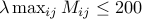 which would be the threshold when numerical problems appear.
Numerical instabilities arise when the elementwise exponential matrix
which would be the threshold when numerical problems appear.
Numerical instabilities arise when the elementwise exponential matrix  has elements that are numerically
  because of insufficient numerical precision caused by a value that is too big. In that case Sinkhorn's algorithm can blow up.
Parallelization
A nice feature of these distances is that their computation is vectorized: the computation of a  distances, whether from one histogram to many, or many to many, can be carried out simultaneously using elementary linear algebra operations. As such, these upper and lower bounds can be computed trivially on GPGPU's.
The implementation provided in Matlab below should also run on your GPU if you have the PCT toolbox. Simply instantiate all input variables on the GPU using the gpuArray command first.
Implementation in Matlab [V0.2b, 21/04/15]
The sinkhornTransport zip file contains an implementation that outputs the upper and lower bounds, as well as the smoothed optimal transport(s) if required.
This zip file contains:
sinkhornTransport.m to compute either:
the dual-Sinkhorn divergences and lower bounds to the EMD of a histogram
 to a family of histograms
 ![[b_1,cdots b_N]](eqs/4674333325135591416-130.png) , as well as their optimal transport maps, with different stopping criteria. We call this the 1-vs-N execution mode.
, as well as their optimal transport maps, with different stopping criteria. We call this the 1-vs-N execution mode. the dual-Sinkhorn divergences and lower bounds of a family of pairs of histogram
 ![[(a_1,b_1),cdots (a_N,b_N)]](eqs/7889273881454671415-130.png) , as well as their optimal transport maps, with different stopping criteria. We call this the N x 1-vs-1 execution mode.
, as well as their optimal transport maps, with different stopping criteria. We call this the N x 1-vs-1 execution mode.
testSinkhornTransport.m to test sinkhornTransport.m with a synthetic example.
Here is what the output returned by this function should look like, with a screencapture below.
>> testSinkhornTransport
***** Example when Computing distances of 1-vs-N histograms ******
Computing 40 distances from a to b_1, ... b_40
Iteration :2 Criterion: 0.68833
Iteration :22 Criterion: 0.25479
Iteration :42 Criterion: 0.10339
Iteration :62 Criterion: 0.063954
Iteration :82 Criterion: 0.042592
Iteration :102 Criterion: 0.030737
Iteration :122 Criterion: 0.023055
Iteration :142 Criterion: 0.02227
Iteration :162 Criterion: 0.021173
Iteration :182 Criterion: 0.019268
Iteration :202 Criterion: 0.016582
Iteration :222 Criterion: 0.013544
Iteration :242 Criterion: 0.010809
Iteration :262 Criterion: 0.0086636
Iteration :282 Criterion: 0.0070937
Iteration :302 Criterion: 0.0060742
Iteration :322 Criterion: 0.0052654
Done computing distances
Display Vector of Distances and Lower Bounds on EMD
Display (smoothed) optimal transport from a to b_29, which has been chosen randomly.
Deviation of T from marginals: 8.5463e-05 1.6837e-17 (should be close to zero)
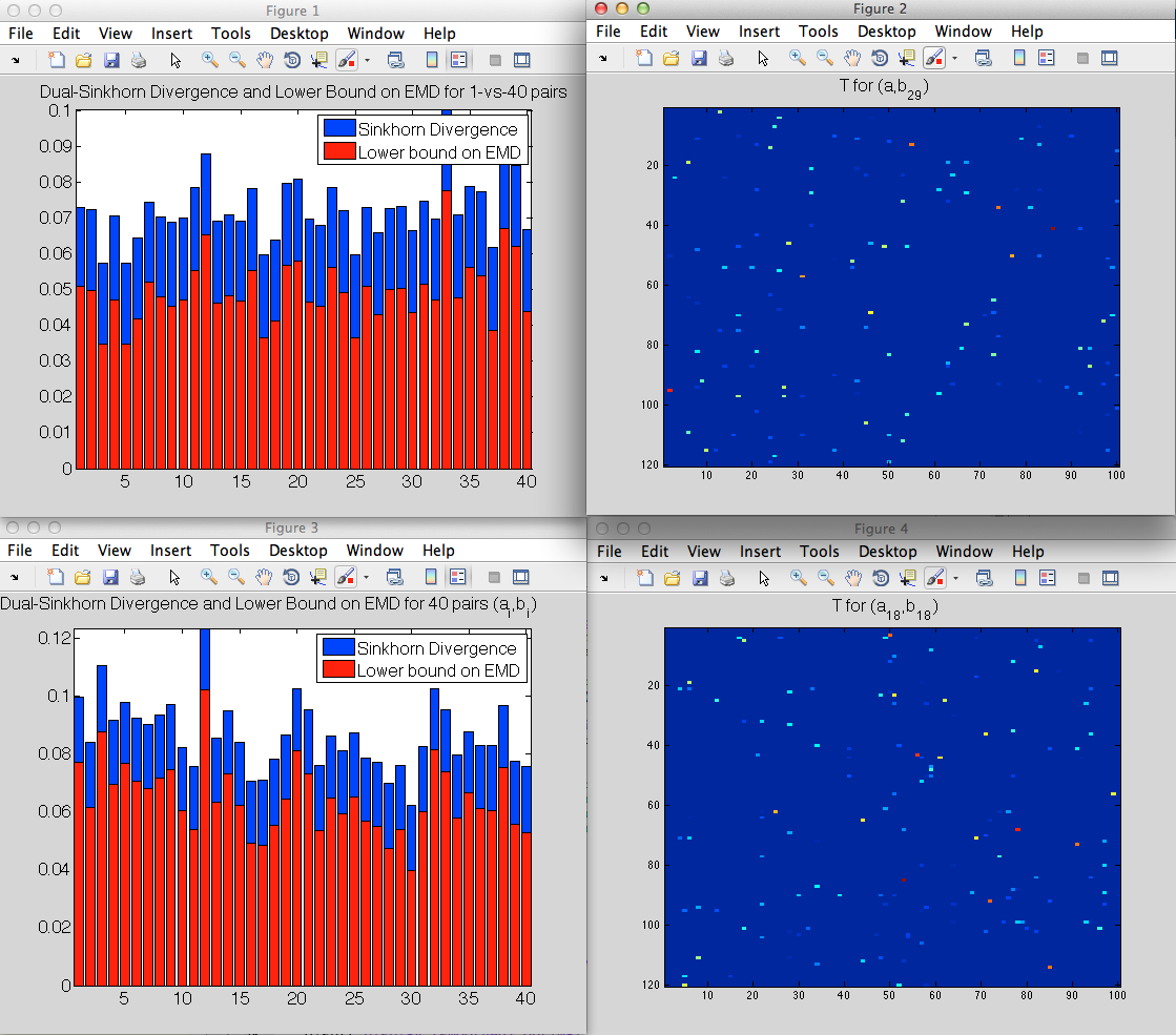
***** Example when Computing N distances between N different pairs ******
Computing 40 distances (a_1,b_1), ... a_40b_40
Iteration :2 Criterion: 0.78215
Iteration :22 Criterion: 0.27524
Iteration :42 Criterion: 0.13837
Iteration :62 Criterion: 0.10322
Iteration :82 Criterion: 0.069004
Iteration :102 Criterion: 0.050905
Iteration :122 Criterion: 0.039758
Iteration :142 Criterion: 0.033102
Iteration :162 Criterion: 0.029907
Iteration :182 Criterion: 0.02512
Iteration :202 Criterion: 0.019432
Iteration :222 Criterion: 0.014022
Iteration :242 Criterion: 0.0097038
Iteration :262 Criterion: 0.0077191
Iteration :282 Criterion: 0.006674
Iteration :302 Criterion: 0.0063764
Iteration :322 Criterion: 0.0062286
Iteration :342 Criterion: 0.0061056
Iteration :362 Criterion: 0.0060178
Iteration :382 Criterion: 0.0058331
Iteration :402 Criterion: 0.0055835
Iteration :422 Criterion: 0.0054018
Iteration :442 Criterion: 0.0053131
Iteration :462 Criterion: 0.005268
Iteration :482 Criterion: 0.0052167
Iteration :502 Criterion: 0.0050954
Done computing distances
Display Vector of Distances and Lower Bounds on EMD
Display (smoothed) optimal transport from a_18 to b_18, which has been chosen randomly.
Deviation of T from marginals: 1.0924e-05 2.3773e-17 (should be close to zero)